How to build a CNN model with Pytorch
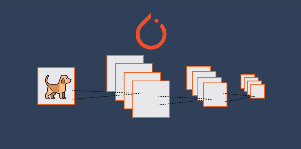 Image credit: Analytics Vidhya
In this post, I will demonstrate how to develop a computer vision classifier to classify images. The dataset used is from insectimages.org. The dataset contains images on beetles, cockroaches, and dragonflies. In this post, I will show how to build a multilayer convolutional neural network (CNN) in Pytorch to classify these images. Then I will discuss how the classifications are made using Shapley Additive exPlanations (SHAP).
Note, in order to leverage powerful computational hardwares(GPU). This demonstration is done on Google Colab. You can access the GPU for free on Google Colab by changing the Runtime to GPU.
1 Data
The data is stored on my Google Drive, and the file structure is organized in a way that train and test data are in two separate directories. Within each train and test directory, each class is organized in different sub-directories.
For example,
Root/train/beetles
Root/train/cockroach
Root/train/dragonflies

Root/test/beetles
Root/test/cockroach
Root/test/dragonflies
To read in the files, torchvision.datasets has a convenient function ImageFolder that can load image data organized in this way.
# Loading necessary libraries

import matplotlib.pyplot as plt
import torchvision
import torch
import torch.nn as nn
import torch.optim as optim
import torch.nn.functional as F
from torchvision import datasets, transforms
import os
import numpy as np
import shap

# making sure we are using GPU
device = torch.device("cuda" if torch.cuda.is_available() else "cpu")
print("device:", device)

# specify file paths
DATA_ROOT = "/content/drive/MyDrive/BIOS823/insects/train"

# transform the data to have height and width 224
transform = transforms.Compose([transforms.Resize(225),
                                transforms.CenterCrop(224),
                                transforms.ToTensor()])


# loading the image data
dataset = datasets.ImageFolder(DATA_ROOT, transform=transform)

# loading data in batches
dataloader = torch.utils.data.DataLoader(dataset, batch_size=128, shuffle=True)
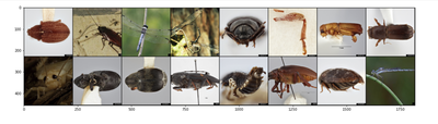
Now, we have the train train data loaded with batch size 128. We want to visualize the data by plotting some sample images. Here is how to do this with matplotlib.pyplot.
# grab a batch of training data
images, labels = next(iter(dataloader))

# choose only 16 to plot
images = images[:16]

# visualize the data
grid_img = torchvision.utils.make_grid(images, 8)
plt.figure(figsize = (20,20))
plt.imshow(grid_img.permute(1, 2, 0))
plt.show();
Notice that I have only loaded the training data, this is because I want to calculate the means and standard deviations of my training data by each RGB channel. Then, I can use the calculated means and standard deviations to normalize both the train and test datasets.
Here the code that I used :
def get_mean_std(loader):

  """Calculate the means and standard deviations of each channel in the dataset.

  Params:
  loader: Pytorch datalaoder object

  Return:
  mean: mean of each channel
  std: standard deviation of each channel
  """

  channels_sum, channels_squared_sum, num_batches = 0, 0, 0

  for data, _ in loader:
    channels_sum += torch.mean(data, dim=[0, 2, 3])
    channels_squared_sum += torch.mean(data**2, dim=[0, 2, 3])
    num_batches += 1

  mean = channels_sum/num_batches
  std = torch.sqrt(channels_squared_sum/num_batches - mean**2)

  return mean, std
mean, std = get_mean_std(dataloader)
Now, we ready to load in both train and test data.
# defining batch sizes

TRAIN_BATCH_SIZE = 128
VAL_BATCH_SIZE = 100

# transform the data and add data augmentation for train data

transform_train = transforms.Compose([
    transforms.ToTensor(),
    transforms.Resize(254),
    transforms.CenterCrop(224),
    transforms.RandomHorizontalFlip(p=0.5),
    transforms.Normalize(mean = [0.5754, 0.5431, 0.4762],
                         std = [0.2613, 0.2716, 0.2998])])

transform_val = transforms.Compose([
    transforms.ToTensor(),
    transforms.Normalize(mean = [0.5754, 0.5431, 0.4762],
                         std = [0.2613, 0.2716, 0.2998])])

TRAIN_DATA_ROOT = "/content/drive/MyDrive/BIOS823/insects/train"
train_dataset = datasets.ImageFolder(TRAIN_DATA_ROOT, transform=transform_train)

VAL_DATA_ROOT = "/content/drive/MyDrive/BIOS823/insects/test"
val_dataset = datasets.ImageFolder(VAL_DATA_ROOT, transform=transform_train)

train_loader = torch.utils.data.DataLoader(train_dataset,
                                           batch_size=TRAIN_BATCH_SIZE,
                                           shuffle=True,
                                           num_workers=4)

test_loader = torch.utils.data.DataLoader(val_dataset,
                                          batch_size=VAL_BATCH_SIZE,
                                          shuffle=False,
                                          num_workers=4)
Note that when we are loading the training data, the transformation applied to the training data include center crop and random horizontal flip. These are data augmentation techniques. Neutral networks are prone to overfit. One of the methods for mitigating overfitting in neural networks is to increase the number of training samples. When dealing with images data, we can increase the number of training data by artificially cropping or flipping some of the training data. In that way, we will have a larger training data that can potential boost the model performance on the test data.
2. Model
Now we have both train and test data loaded, we can define the model for training. Here we want to construct a 2-layer convolutional neural network (CNN) with two fully connected layers. In this example, we construct the model using the sequential module in Pytorch. To define a sequential model, we built a nn.Module class. Here is the code to build it.

class Net(nn.Module):
    def __init__(self):
        super(Net, self).__init__()

        self.conv_layers = nn.Sequential(
            nn.Conv2d(3, 8, kernel_size=5),
            nn.MaxPool2d(2),
            nn.ReLU(),
            nn.Conv2d(8, 16, kernel_size=3),
            nn.Dropout(),
            nn.MaxPool2d(2),
            nn.ReLU(),
        )
        self.fc_layers = nn.Sequential(
            nn.Linear(16*54*54, 120),
            nn.ReLU(),
            nn.Dropout(),
            nn.Linear(120, 84),
            nn.ReLU(),
            nn.Linear(84, 3),
            nn.Softmax(dim=1)

        )

    def forward(self, x):
        x = self.conv_layers(x)
        x = x.view(-1, 16*54*54)
        x = self.fc_layers(x)
        return x
After defining the model, we can check the model by printing out the exact model architecture.
model = Net()
print("Model Architecture:")
print(model)
We could test the mode by passing some randomly generated tensor to check if we have made any mistake calculating the dimensions of the output from the previous step correctly. For example,
input_size = (128, 3, 224, 224)
sample = torch.rand(size = input_size)
out = model.forward(sample)
print(f"* Input tensor size: {input_size}, \n* Output tensor size: {out.size()}")
Here, we generated 128 tensors of dimension 3 X 224 X 224 to pass in the model. And we expect to see the final model output to have dimensions of (128, 3). This is because we have 128 different tensor and each tensor has 3 probabilities associated with three different classes. After we are sure that the model is implemented correctly, we can put the model to GPU and start training.
num_epochs = 10
def train(model, device, train_loader, optimizer, epoch):
model.train()
for batch_idx, (data, target) in enumerate(train_loader):
data, target = data.to(device), target.to(device)
optimizer.zero_grad()
output = model(data)
loss = F.nll_loss(output.log(), target)
loss.backward()
optimizer.step()
if batch_idx % 5 == 0:
print('Train Epoch: {} [{}/{} ({:.0f}%)]\tLoss: {:.6f}'.format(
epoch, batch_idx * len(data), len(train_loader.dataset),
100. * batch_idx / len(train_loader), loss.item()))
def test(model, device, test_loader):
model.eval()
test_loss = 0
correct = 0
with torch.no_grad():
for data, target in test_loader:
data, target = data.to(device), target.to(device)
output = model(data)
test_loss += F.nll_loss(output.log(), target).item() # sum up batch loss
pred = output.max(1, keepdim=True)[1] # get the index of the max log-probability
correct += pred.eq(target.view_as(pred)).sum().item()
test_loss /= len(test_loader.dataset)
print('\nTest set: Average loss: {:.4f}, Accuracy: {}/{} ({:.0f}%)\n'.format(
test_loss, correct, len(test_loader.dataset),
100. * correct / len(test_loader.dataset)))
# put the model to GPU device
model = Net().to(device)
optimizer = optim.SGD(model.parameters(), lr=0.01, momentum=0.5)
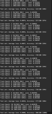
for epoch in range(1, num_epochs + 1):
train(model, device, train_loader, optimizer, epoch)
test(model, device, test_loader)
After 10 epochs of training, the model reaches 100% accuracy of the validation set!
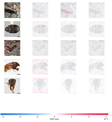
Shapley Additive exPlanations (SHAP)
Shapley value is a concept based on cooperative game theory that measures how much does a feature value contribute to the output across all possible coalition. Shapley Additive exPlanations (SHAP) is a modification of Shapley values by adopting ideas from local surrogate models (LIME). When we are dealing with image data, each pixel is typically treated as a feature. Computing for Shapley values is computational expensive. In this case, I used the Deep Explainer in the SHAP Python package. Deep Explainer is used to approximate SHAP value s for deep learning models, where SHAP values are approximated using a selections of backdrop samples.
# since shuffle=True, this is a random sample of test data
batch = next(iter(dataloader))
images, _ = batch

background = images[:60]
test_images = images[4:9]

e = shap.DeepExplainer(model.cpu(), background)
shap_values = e.shap_values(test_images)

shap_numpy = [np.swapaxes(np.swapaxes(s, 1, -1), 1, 2) for s in shap_values]
test_numpy = np.swapaxes(np.swapaxes(test_images.numpy(), 1, -1), 1, 2)

# plot the feature attributions
shap.image_plot(shap_numpy, test_numpy)
Refer to the complete code and notebook here!